
The idea was simple. We place evenly spaced markers around the edge of a circle, and then draw lines between them. If you follow the blue lines, you can see they start at a marker, miss a marker, and end at the next marker. The yellow lines skip two markers.
Could we create some algorithmic art based on these ideas?
Going Around a Circle
We need a mathematical way to move around a circle in evenly spaced steps. How can we do this? The easiest way is to start with how we naturally think about following the outline of a circle - we naturally think about turning in even steps. That means we increase our angle of turn in even steps. We're familiar with angles to measure the amount of turn from our time at school. The following shows some examples of counting angles in degrees.
Computers, and programming languages like Processing and p5js, internally work in terms of horizontal and vertical (x, y) coordinates. That means we need to translate our moving around a circle by counting the angle, into (x, y) coordinates. Luckily there is some maths that helps us.

The maths allows us to translate from the world of angles into the world of (x,y) coordinates. You can see from the diagram above that point P is at an angle A, around a circle which has radius R. what we want is to be able to say how far across, x, and how far up, y, that point is. The maths tell us how to do that:
- x = R cos(A)
- y = R sin(A)
The cos() and sin() are mathematical trigonometry functions, which you can find on most calculators, and in many programming languages, including Processing.
If we count up the angles A from 0 to 90 degrees in steps of 10, and use that trigonometry to calculate x and y coordinates, and mark those points with little red dots, we get the following.

That shows the maths works. If we carried on counting beyond 90 to 360 degrees, we'd get a full circle of dots.
Skip Step Patterns
The following shows the idea of drawing lines between these markers, but missing a few markers, like our original doodle.
You can see how we can count up the angle in steps, just like we've done, and that point can be the start of the line. You can also see that the end of the line is at a point that's just a few angle steps ahead. The diagram shows the point 6 steps ahead. If we were counting the angle up in steps of 10 degrees, the end point would be at (angle + 60) degrees.
If we repeat this process of drawing lines, we can create nice patterns like the following, which shows 2 overlaid patterns created from different skip steps.

We can have a lot of fun varying the number of skip steps to create different patterns. But let's do something even more ambitious.
Gears
Have a look at the following diagram. It shows a new imaginary circle centred at point P. That smaller circle, shown green, has a point Q that goes around its edge, just like point P went around the big circle's edge.
You can also see that we've set the point Q to go around faster than point Q. Whenever point P is at an angle A, point Q is further along at point 2A. That's just a choice we've made for now. There is some basis for this - this systems works like gears, where the smaller cog turns faster than the larger cog.
What would happen if we plotted points Q as they went around that circle? We can calculate the (x,y) coordinates of Q by realising we can calculate how far Q is from P just like we did before.

We can use the same trigonometric equations to tell us how far along x2 and up y2 the point Q is from P. You can see from the diagram the coordinates of Q are then (x1 + x2, y1 + y2). We've renamed the location of P to be (x1, y1).
Here's the result.

That's interesting, but not really that exciting. What happens if we make Q go faster at 5A not 2A?

That's much more interesting. In fact we have spend hours tweaking the angular speed of Q to get different patterns.
Let's not be satisfied with that though. Look at the following diagram.

Now we have yet another, even smaller red circle attached to the medium sized green one. That one has a point S that turns around the centre which is point Q. And we know point Q turns around point P. Here's we've chosen to have point S turn even faster at an angular speed of 15A, that is fifteen times faster than point P goes around the big circle.
We can do the same maths to work out the position of point S. Here's the result of setting Q to speed 5A and S to speed 20A.

That's an interesting pattern. It loops in on itself, which we expect as the smaller circles create tighter loops, along a broader trajectory set by the bigger circles. The dots make it harder to see the fine detail, so let's increment the angle A in smaller units of 0.1 degrees - that's a tiny turn! We can also set the red dots to be translucent - which helps to see more detail when things get overcrowded. Here it is again.

Much better. We can see the denser areas where the points are closer together because the point S is moving more slowly.
Now, let's do one more enhancement. Let's take the angle for each of the points on the large, medium and small circles, and add some variation to them. So if we take an angle A for point P, we can create several new versions of this by adding a small amount to it. If we added 1 degree to it, nine times, we'd get nine new angles, A+1, A+2, A+2 ... A+9. Let's call this new additive parameter t, which we can add to each of the angles for points P, Q and S. The following diagrams shows the idea.
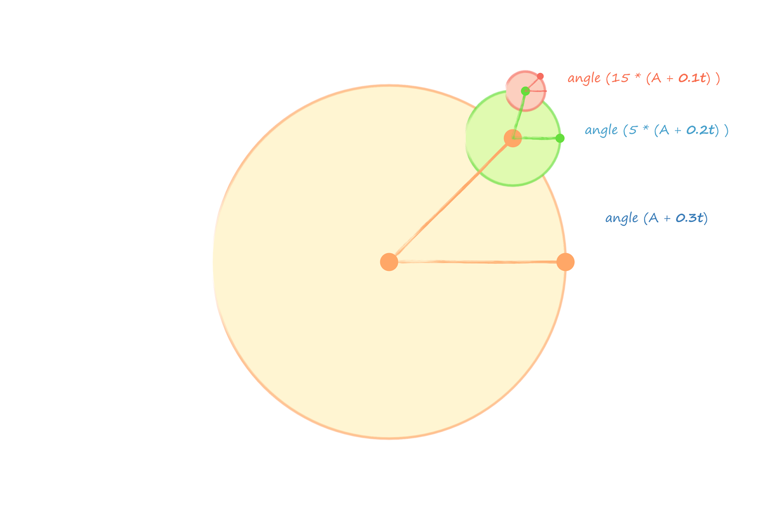
You can see that several versions of P are calculated at angle (A + 0.3t) where t varies, say from 0 to 100. Similarly, point P has versions with angles 5(A + 0.2t), and point S has 15(A + 0.1t). You can see that we've multiplied the t by quite small fractions - that's just arrived at through experimenting with what works and what doesn't.
Plotting the points that correspond to the point S, for every variation that comes from these little additions should give some interesting results.
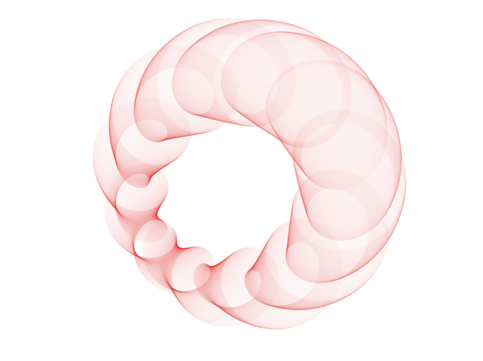
This one is based on the same pattern above with angular speeds: P at A, P at 5A and Q at 15A, and the angles for P varied by 0.1t, Q by 0.2t and S by 0.3t.

It's really nice! The source code is at https://www.openprocessing.org/sketch/474017. Feel free to copy and change it.
Experimenting with both the angular speeds, and also the angle variations give us a wide variety of interesting, natural forms. This one looks very ribbon like.

A simpler one.

This one looks very cloudy.

I really like this one, which is also online at https://www.openprocessing.org/sketch/476269. It evokes some kind of alien sea creature!
This blog is adapted from a section of my upcoming gentle introduction to algorithmic art - Make Your Own Algorithmic Art, which starts from no assumed expertise in coding or maths, and goes gently from there.
Join in with the Algorithmic Art meetup group, which meets monthly in London.
Nice! Your post reminded me of the epicycloids used before Kepler trying to explain the orbits and movements of the planets.
ReplyDeleteWaiting for your new book to become available, I enjoyed very much "Making your own neuronal network"
Best Regards.
Thanks Luis - I will have to read more on Kepler and epicycloids!
Delete